Abstract :

This study aims to gain insights on various issues that surround stock market volatility. For this purpose, more than forty empirical studies have been examined to critically assess issues like, heteroscedasticity, asymmetric effect, risk-return framework, spillovers and forecasting accuracy. With the help of time-series plots, the study demonstrates in layman terms how mean-reversion, clustering and heteroscedasticty exhibits in stock market volatility. This study finds GARCH variants to have a wider applicability in the modelling of volatility persistence despite fearing poorly in evaluation against naive methods like realised volatility, EWMA. The asymmetric effect doesn’t seem to be as strong at firm level as it appears at the broad market index level. Evidence of statistically weak relation between conditional volatility and expected returns raises questions about accuracy of the volatility measures plugged for testing the relation. In case of spillover effects, immunity/propensity of a market to face/generate systemic shocks from/to other markets is likely to be determined by level of market development. On the whole, empirical findings lack a general consensus on the volatility properties. This may be due to sensitivity of different findings to the models and frequency and time length of sample data used by the study.

Keywords :

stock market, heterscedasticity, asymmetric effect, conditional volatility, GARCH.

1. Introduction

Volatility in stock markets is very wellfounded in the basic framework of Efficient Market Hypothesis (EMH). Precisely, EMH implies that markets are efficient and hence, stock prices and stock returns are fully reflected in the market trends. In an ideal situation, if this be the case, the entire information content that backs the market should smoothen the process of adjustment in the market. EMH sees volatility in returns as a response of the economic agents to the unexpected information. If the perception of agents about the impact of the information is of temporary nature, then the volatility in the market will be low. Conversely, if agents perceive the impact of the information as permanent, then in that case, volatility may be higher. Thus, volatility occurs due to the rational expectations of the agents in their valuation of financial assets. However, in practice, information is characterised by its occurrence in lags, spikes and asymmetric effects, all of which leads to a situation where markets no longer remain perfectly efficient. Primarily, this is the cause of volatility. Some amount of volatility, however, is necessary in financial markets. Stock markets cannot attract investors, arbitrageurs and other participants if they remain completely docile. This is because variations in the stock prices/returns forms the basis of incessant trading in these markets. Without such a trend, markets would not have the necessary buoyancy to keep itself afloat. In the absence of this buoyancy, markets would tend to be flat and sterile. Hence, the interested agents would not have the incentive to enter and exit the market as and when their expectationsare met or belied. Therefore, it is evident that some amount of volatility is necessary for retaining the trading environment. However, large volatility and unexpected trends in volatility don’t auger well for the stock market. In the recent times, therefore, there has been a great deal of interest generated in stock market volatility and stock returns. Some of the prominent question that have been raised in this regard are:-

• Does stock market volatility remain constant over time?
• Does volatility in the stock markets persist?
• Is there an asymmetric reaction by the volatility to the news or information content? Keeping these issues in view, the theme of this paper is to lay out the literature that explores the nature of the volatility and its relationship with stock returns.For this purpose, we examined over forty research papers to present a concise view of various issues surrounding the concept of volatility. The rest of the study is summarised as: the second segment takes up discussion on theoretical background, followed by segment third that presents the comprehensive extract of review effort under six sub-segments, segment fourth gives critical tinge to the findings from the review and finally segment fifth summaries with a conclusion note.

2. TheoreticalBackground:

Investing in stock markets requires understanding of both return as well as risk concepts. While return is considered as a reward of investing and the risk is the amount of potential loss associated with such investment. In finance theory, risk and return should have a positive relation, i.e., increase in risk should lead to increase in the expected returns. However, due to certain reasons, this theorem in reality sometimes doesn’t hold good. The term, “return” literally means the rate of change that occurs between two time periods in the value of an investment and the risk is the potential variability or volatility in that return. Stock return is unique from returns of other types of investments because of the implication of continuous compounding concept. Such a nature of stock return requires its measurement from a natural logarithmic scale. If r_t be the return at time t and p_t be the price of a stock at time t , then logarithmic return of the stock may be expressed as:

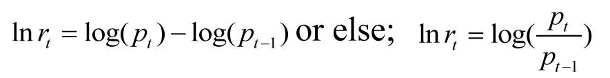
The dividend component of the return is not considered here solely for being insignificant when fragmented into daily basis. Using logarithmic scale in case of stock returns has many advantages. The use of such a scale makes returns additive over time and can also lead toapproximation of return distribution to normal. For a pretty long time, volatilitywas considered to be time invariant. Moreover, volatility was believed to be conditional upon market maintaining a linear relationship with the expected returns on a particular stock. Most of the previous empirical studies attempted to study the trade-off between expected return and risk assuming unconditional distribution of an asset’s returns. All this was consistent with the assumptions of EMH, however, over past, many anomalies to such theories have been found to exist in case of volatility and its relation with a stock’s returns. Application of the GARCH-M4 model for testing pricing efficiency of financial assets is just a crucial breakthrough because it allows mapping of the conditional variance5and expected returns, henceallowing risk(volatility) to be time variant so asto explainin a much better way interdependence of risk and return components in a financial asset or portfolio. This procedure abolished earlier restrictive assumptions that include linearity, independence, and unconditional variance assumed by the earlier models. Considering volatility as constant over time is now considered as a vague argument. Even the beta, which is a measure of risk under CAPM framework is now being widely recognisedas phenomenon that varies over time.

Let’s examine cursorily a few of the arguments that are now raised in favour of concept of volatility. It is widely being believed that volatility is time variant. Not only that, it is also being argued that volatility appears in clusters, though does revert to its mean value over a longer period of time.

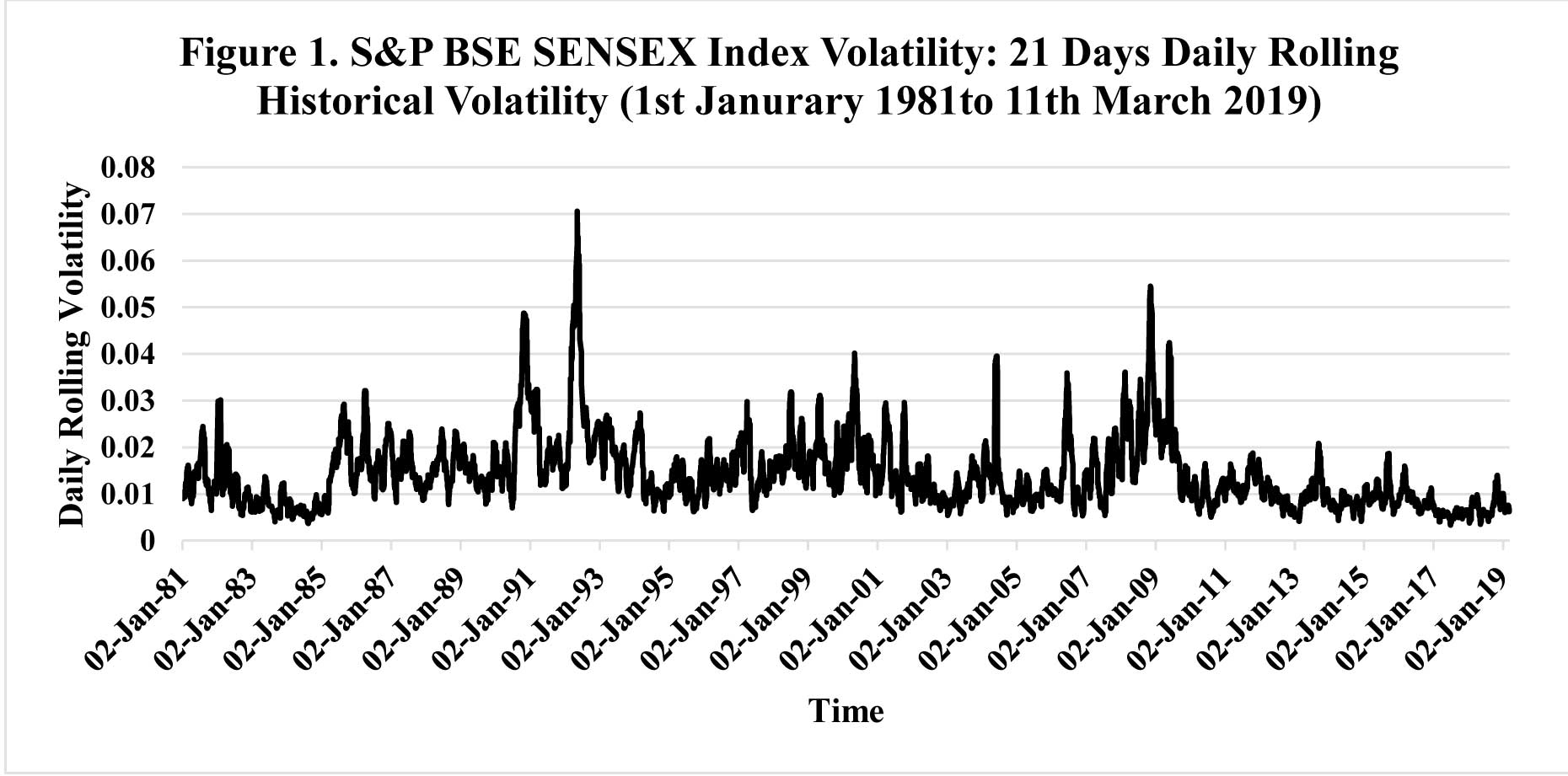
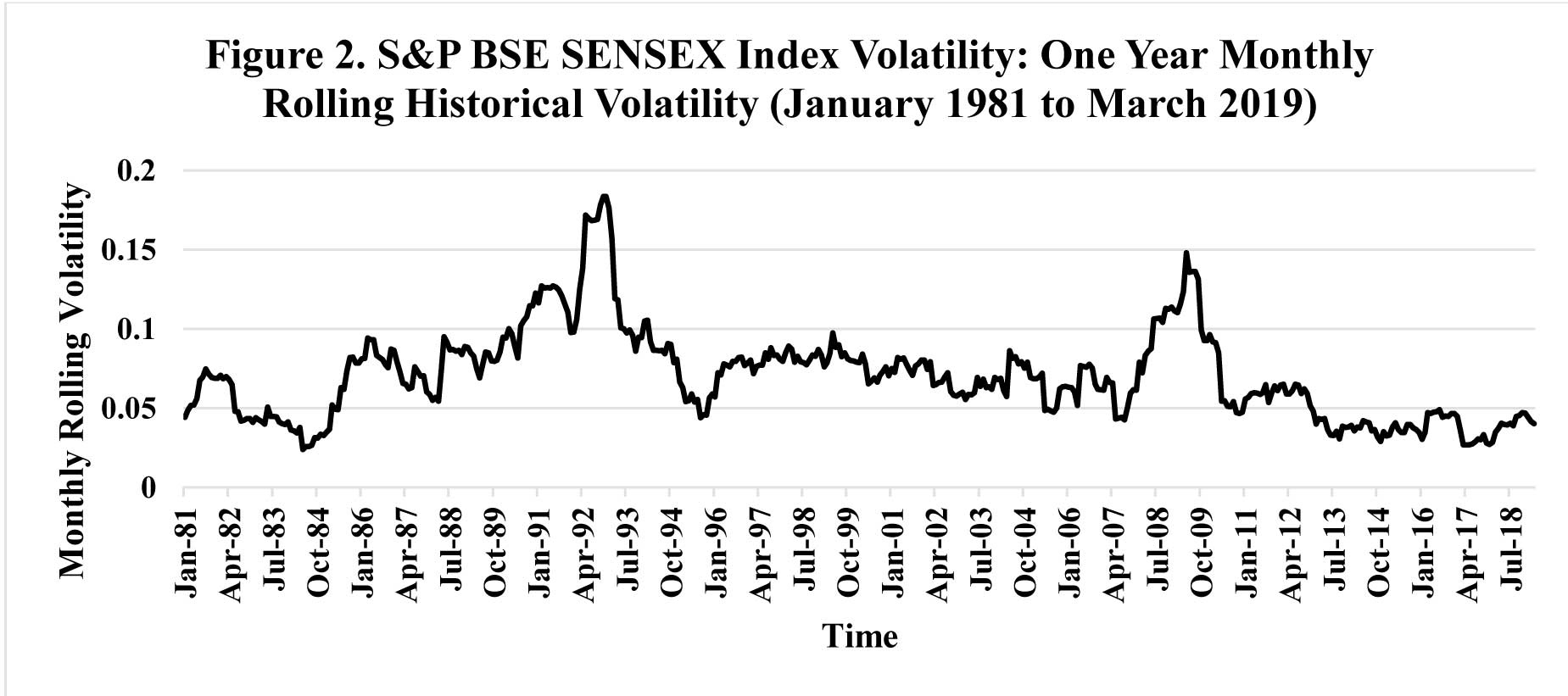
To illustrate these properties of stock return volatility, volatility of S&P BSE SENSEX6 on daily and monthly basis using traditional standard deviation method has been shown in Figure 1 (above) and Figure 2 (below). Figure 1 demonstrates behaviour of 21 days daily and the Figure 2 shows 12 months monthly rolling standard deviation of the S&PBSE SENSEX index returns for last 38 years7. A look at these charts can lead to understanding of some interesting facts about the behaviour of volatility at the broad stock market level. The line on the graph in Figure 1 reflectsvolatility for each rolling 21 day period starting in 2nd January 1981 and moving with each dayup to the present, i.e., 11th March 2019. Similarly, second graph shown as Fig. 2 reflects volatility for each rolling 12 month period starting in January 1981 and moving with each month up to the present, i.e., March 2019. These graphs help in understanding phenomenon of stock market volatility in several ways. First of all, we come to the understanding that volatility itself is volatile; i.e., it cycles erratically over time. Second, in these graphs it can be seen that periods of high volatility is followed by periods of high volatility and also period of low volatility often followsperiods of low volatility, thus supporting the argument that volatility projects clustering patterns.

Third, volatility tends to hover around the averagemost of its time and it doesn’t show any tendency to drift upwards permanently, i.e., although both of the graphs show disturbances in volatility over time, yet when we look at the line in whole it gives a flat depiction. In the long run, volatility is following a mean-reverting process. Now, put technically, both of these graphs project volatility clustering8, a phenomenon under which large changes in volatility are followed by large changes and small changes in volatility are followed by small ones. In other words, volatility appears to arise in bunches. High or mounting volatility often corresponds to plunging markets; low or falling volatility corresponds to good markets. Given these unique characteristics of the stock market return movements as evident from these graphs, modelling volatility becomes a challenging task. The Autoregressive Conditional Heteroscedasticity or ARCH9 and Generalised Autoregressive Conditional Heteroscedasticity or GARCH10 models are specifically meant to deal with these issues related to stock returns volatility.

3. Empirical Research on Volatility in Stock Returns:

This segment presents the empirical review of the literature on volatility of stock returns. First, empirical research on the heteroscedastic character of stock returns volatility is examined. Many studies have shown that volatility of stock returns varies over time. However, frequency of a random variable whose volatility is intended to be measured plays a great role in shaping its associated probability distribution, and hence choice of parameters in a conditional volatility modelling set up. Some studies have shown volatility to exhibit clustering patterns and persistence. In the second sub-segment of our review work, literature on risk-return trade-off ability of the GARCH models has been examined. In the third and fourth sub part, two important stylised facts, asymmetric volatility effect, i.e., the potential of volatility to respond to the nature of news or information differently and spill-over effect, i.e. the ability of volatility to transcend over to other markets and national geographies has been thoroughly reviewed. The fifth part of the review segment discusses the forecasting ability of GARCH models.

3.1 Heteroscedastic nature of Volatility:

It is now an established fact that volatility of stock market returns varies over time with clustering effects. The idea of volatility clustering which implies that, “large changes in volatility tend to be followed by large changes, of either sign, and small changes in volatility tend to be followed by small changes“, was first documented by Mandelbrot (1963) and later on it was further elaborated by Engle (1982) and Bollerslev (1986) with the introduction of Autoregressive Conditional heteroscedasticity (ARCH) and Generalised Autoregressive Conditional heteroscedasticity (GARCH) models. Cont (2007) while using a simple agent-based model has explained the phenomenon of volatility clustering through the activity of market participants on the basis of news arrival process. The agent based models explain the behavior of prices in terms of the trading rules adopted. The author has stated that significant autocorrelation function of absolute returns over several lags decaying slowly to zero is the typical manifestation of the volatility clustering phenomenon. Demetrescu (2007) states that market participants individually often perceive risk of a stock given by volatility, differently. However, the general their perception about risk of a stock is influenced by market risk. Thus when there is a perception of high market risk, the realized volatility will also be high. On the other hand, since volatility is assumed to be time varying, modeling the same on the basis of historic data would lead to a higher or lesser expectation of current volatility and thus a higher or lesser perception of market risk. Demetrescu (2007) thus stated that “it is a plausible scenario to observe volatility clusters simply because everybody expects them”. Schmitt and Westerhoff (2016) have attributed the volatility clustering phenomenon associated with stock returns to the herding behaviour of speculators. During periods of high uncertainty, the market trading rules becomes less heterogeneous as speculators observe other speculators on trading rules. This results in high volatility since the prices are adjusted strongly by the market maker who faces a less balanced excess demand. However, during periods of low volatility in the stock market, the trading rules adopted by speculators are relatively more heterogeneous, since speculators trade independent of each other. The market maker facing a balanced excess demand eventually adjusts prices less forcefully and as such volatility remains low. Gaunersdorfer and Hommes (2007) have stated that even though price changes are unpredictable, absolute changes or squared returns are predictable implying that small changes are followed by small changes and large changes are followed by large changes. Banumathy and Azhagaiah (2015) found that volatility exhibited long memory or persistence in the S&PCNX Nifty daily returns in Indian stock market which indicated relatively lesser role of new shocks in shaping the volatility than the past volatility. Theirresultsshow presence of volatility clusteringinthe the Indianstockmarket. Goudarzi and Ramanarayanan (2011) in their study show evidence about volatility clustering and leptokurtosis11associated with stock returns in the Indian stock market using conditional return volatility of BSE500 index returns. Karmakar (2005) modelled long-run volatility of market index returns in the Indian stock market for a period of 45 years using GARCH (1,1) model and found evidence about the persistence of volatility in the Indian Stock market. In another study, Karmakar (2007) examined the volatility properties of daily stock index returns of S&PCNX Nifty in India using GARCH (2,1) model and found the evidence of time varying volatility that exhibits clusterswith high level of persistence and predictability in the Indian stock market. Padhi (2006) examined the stock market volatility in India for the period of January 1990 to November 2004 using daily stock price data of five indices (representing five broad sectors) and four companies from each sector comprising twenty in all from various sectors of the chosen indexes. The study observes that volatility as a whole in the sample companies is changing over time. The study established presence of volatility persistence (clustering) in the Indian stock market using GARCH models (with varying lag length) for different sample companies. Sah (2011) examined the behaviour of index return volatility in India in context of the US sub-prime crisis for the period extended from 1st April 2000 to 31st March 2010 using daily close prices of NSE S&PCNX Nifty index. The author argues that returns of the index follow leptokurtic distribution and their volatility exhibits clustering. The results of the GARCH (1,1) model reveal high persistence of volatility in the sample index returns.

3.2 Risk-return trade-off:

Risk-return trade-off is considered as the centre piece of the entire stock return volatility empirical research. Under ARCH/GARCH paradigm, time varying volatility as a measure of risk is believed to have a trade-off with the time varying expected returns of the stocks. A few studies have been reviewed where in results about establishment of relationship between the duo has been mostly found statistically not significant. Banumathy and Azhagaiah (2015) examined the relationship between the conditional variance and expected return of index returns inIndian stock market using GARCH-M model documenting evidence of a statistically insignificant relationship.However, presence of a significant intercept term in the model gave indications about the existence of abnormal returns or returns due to other factors than the market. Karmakar (2007) examined the risk-return trade-off of the daily stock index returns in the Indian stock market using GARCH-M (2,1) modeland found a positive but statistically insignificant relation between the conditional variance and the expected returns. Padhi (2006) investigated time varying risk-return trade-off in the Indian stock market both at the aggregate level as well as firm level using data of five sectoral indices and twenty individual stocks comprising of four stocks from each index. The author found mixed results with majority of the cases revealing a positive risk-return relationship with significant statistical support. Shin (2005) studied the stock return and volatility in the 14 emerging markets using weekly stock price data. Applying both a parametric and a flexible semi parametric GARCH-M model, the study found a positive relationship prevails for the majority of the emerging markets, which is though statistically insignificant in most of the cases.

3.3 Asymmetric Volatility effect:

The asymmetric property of volatility first of all documented by Black (1976) suggests that bad news has a greater impact on volatility than the good news. It implies that there is a negative correlation between stock returns and volatility and the correlation is more significant in case of negative returns. Dutta (2014) states that for volatility modelling, the model should be such in which the asymmetric impact of news should be taken care of. However, the traditional GARCH model does not take into account differential impacts of good and bad news on stock return volatility. The introduction of the Exponential-GARCH by Nelson (1991) has led to better modelling of conditional stock market volatility. The GJR-GARCH named after the econometricians Glosten et al. (1993) who introduced it, also deals with the problems of the conventional GARCH in terms of modelling of asymmetric impacts of news on stock return volatility. This property of volatility has been often described in research as the leverage effect. Christie (1982) argues that with a decline in price, the value of market equity reduces compared to the market value of debt, as such, increasing the financial leverage of the firm. This implies that the risk of the firm increases, as such, increasing the volatility of the firm. Further, any increase in firm’s risk should coincide with higher expected return implying a price drop, hence increasing volatility. Mishra and Rahman (2010) have found that while Japanese stock market is impacted more by negative news, however, in the Indian stock market the influence of positive news is more. Goudarzi (2011) has stated that negative returns are generally associated with upward revisions of conditional volatility. This implies that the market participants are generally risk averse and as such respond more to bad news. The author in order to investigate this phenomenon conducted a study on the BSE500 price index using EGARCH and TGARCH models, and observed that BSE500 returns series reacts to the good and bad news asymmetrically. The asymmetric response of volatility to the news would connote that the adverse shock (news) would have a greater impact on volatility than a favourable shock (news), indicating that the sign of the news matters when a new flow of information drives volatility. Hence, arrival of bad news in the market would result in the volatility to increase more than good news. Gogia (2012) has pointed out that “the leverage effect hypothesis is a down market effect since the effect is much stronger when the market is falling”. However, the argument placed is that the phenomenon is more pronounced for indices than for individual stocks. Gupta (2014) and Sood and Saluja (2006) have separately established the presence of leverage effect in the Indian stock market using Threshold (T-GARCH) and Exponential (E-GARCH) models. Banumathy and Azhagaiah (2015) modelled index return volatility in India by applying EGARCH-M and TGARCH models to confirm the presence of a statistically significant leverage effect in the Indian market. Bose (2007) in respect of both intra and inter-day futures and spot index returns argues that bad news at any given time pushes up volatility in the next period by about three times as much as a good news of similar magnitude. Hence, in presence of a high degree of asymmetry in news impact, it would be difficult to reverse high volatility in times of sharp market retreats by infusing positive policy news into the market. Karmakar (2005) found using daily return data of 50 individual stocks of the Nifty that only eight out of fifty companies exhibited significant leverage effect and as such needed an asymmetric GARCH model, such as EGARCH to capture their unique nature of volatility. This is a crucial finding at the micro market or firm level.In another study Karmakar (2005) found that index return volatility in India for pre-1990 period (post-1990 period) exhibit a significant positive (negative) asymmetric effect. Put differently, bad news slightly reduces the volatility during the pre-1990 period, while it increases the volatility substantially for the post-1990 period indicating a reversal of the well-known asymmetric effect of volatility. In yet another study, Karmakar (2007) found using EGARCH (1,1) model that conditional variance of S&PCNX Nifty index returns is an asymmetric function of previous period innovations in which a negative shock causes volatility to go up more than a positive price shock of the similar size. Okicic (2015) analysed the stock returns and volatility in the Central and Eastern European (CEE) region through EGARCH and GJR models and found existence of the leverage effect in case of stock markets from the CEE region, which indicates that negative shocks increase the volatility more than positive shocks. Sah (2011) examined stock return volatility in India during US sub-prime crisis using TARCH model to notice evidence of asymmetric volatility effect in the Indian stock market. Shin (2005) studied the stock return and volatility in the 14 emerging markets and found little evidence for asymmetric volatility argument that stock return volatility should be negatively correlated with stock returns in the given sample. These findings lead to the understanding that evidence on asymmetric effect in stock market volatility is still paradoxical in nature and hence calls for a thorough revisit.

3.4 Volatility Spillovers:

Due to the integration of world economy during 1980’s through globalization and liberalization including formation of various regional trading blocs, the flow of information started to transcend across national stock markets at a greater pace than ever before. Thus the transmission of stock market volatility, containing stock market information, across countries has become inevitable. The empirical research in the area has emphasised both stock return as well as volatility spillover effects between national stock markets. Spillover effect makes a market more vulnerable to external crisis rather than internal economic disruptions, hence, its understanding assumes weight. Bhar and Nikolova (2007) provide evidence of a positive return spillover from world index to all the BRIC countries, a positive volatility spillover effect from world index to Russia, Brazil and India and a negative volatility spillover effect from world index to China. Singh et al. (2010) have analysed the volatility spillover effect across India and most of the major world economies including United States, China, Japan and Germany to put on record that Asian markets are more integrated than European or US markets and that returns and volatility influences are prevalent more in the former than in the later two markets. They also found evidence of impact of Japanese volatility on the Asian markets which itself is influenced by the volatility from US and European markets. Overall, their results support the presence of positive volatility spillover from other markets to the Indian market. Mukherjee and Mishra (2010) investigate into both contemporaneous and the lagged (with a lag of 1 day) intraday as well as overnight information spillover between 12 stock exchanges chosen from Asian region representing both developed and emerging markets of these regions. They find evidence of a bi-directional contemporaneous intra-day return spillover between India and most of Asian counterparts and contemporaneous spillover of intraday volatility is stronger from other foreign markets to India only, while as dynamic intraday spillover among India and its major Asian counterparts are not found to be stronger. Among various Asian markets, Hong Kong, Korea, Singapore and Thailand cause significant flow of market information to Indian market, while as stock markets in Pakistan and Sri Lanka are strongly influenced by the movements in the Indian stock market. Similarly, overnight volatility spillover effect has been found significant in case of most of the Asian countries except Taiwan. Conversely, all Asian markets except china and Malaysia have overnight return and volatility spillover effects caused by Indian stock market. Jebran and Iqbal (2016) using GARCH (1,1) have revealed absence of any spillover effect of volatility across Indian and Chinese stock markets. However, bidirectional and unidirectional spillover effects have been established across other Asian markets. Bose (2007) found a bi-directional spillover of volatility effect across S&PCNX Nifty stock index and S&PCNX Nifty futures index using asymmetric TGARCH method in case of inter as well as intraday volatilities. However, degree spillover from the futures to the spot market is higher and during the day, the contemporaneous spot market volatility seems to have a greater effect on the futures market volatility. Pandey and Kumar (2011) observe that returns in the Indian stock market are getting effected by china's market and by its own lagged returns and volatility of the Indian market is getting effected by Germany, Japan, China and Indonesia. The volatility of every other country's market measured as one day lagged volatility is affecting returns in the Indian stock market. Volatility of Indian stock market is also affected with previous day volatility of its own and volatility of stock markets of Japan, China, Singapore and Indonesia. Overall, the study establishes a uni-directional volatility spillover effect from most Asian markets to the Indian market. Peng (2017) using Bi-GARCH model found that returns on both TAIEX and NIKKEI were substantially influenced by their lagged period returns. The past returns on NIKKEI influenced significantly current period returns of TAIEX, yet there was no such influence flowing from past returns of TAIEX to the current returns on NIKKEI index. Both market are intertwined through a strong mutual volatility spillover effect and a mutual price leading effect with each other. Further, the two stock markets are more sensitive to falling rather than rising trends of each other, implying that there is a mutual tendency between these markets to crash due to a retreat in the counterpart market. Wang et al. (2005) found evidence of significant return spillover from the US and Japan to India, Pakistan, and Sri Lanka. Further, at different levels of statistical significance, volatility spillover effects are also observed from US to Sri Lanka and Japan to Pakistan and US to India. The asymmetric volatility transmission mechanism operates from the US stock market, i.e. to the Indian and Sri Lankan stock markets signifying that negative innovations in US equity prices increase volatility in considerably more than positive innovations in India and Sri Lanka. The study observed huge post crisis spillovers effect from US to India and Sri Lanka, yet no volatility spillover during the period of Asian Crisis is traced. Interestingly, before crisis, Japanese stock market is effecting the volatility spillover, but post crisis, US stock market bears greater impact on the volatility of three small south Asian markets.

3.5 Volatility Forecasting:

The efficiency of volatility forecasting techniques has evolved over time. A time series that exhibits clusters or persistence is believed to have strong predictive strength. GARCH models are designed to capture inconsistencies in the behaviour of a time series of returns. As such, the forecasting ability of volatility of stock returns by GARCH model has been widely debated in the empirical literature. Kumar (2006) in his study evaluates various volatility measures like, random walk, historical mean, moving average, simple regression, exponential weighted moving average and simple and higher order GARCH using both stock market and foreign exchange rate data of the Indian market. The study evaluates different competing models on the basis of two classes of evaluation measures – symmetric and asymmetric error. The study concludes that EWMA12 model fears well in the stock market while GARCH model is appropriate for modelling volatility in the forex market. Nath and Dalvi (2008) examine suitability of volatility measures in the Indian stock market using intraday (minute to minute) and daily logarithmic returns of stock index S&P CNX NIFTY. The study estimates and evaluates seven different measures of volatility. The authors argue that realized volatility measures given by sum of squared returns from high frequency data, the sum of squared returns from high frequency data scaled by the Merton scalar (2002) and standard deviation of the 1-minute high frequency returns time scaled by "N=335" perform better in comparison to the GARCH, IGARCH and end of day return squares. Yu (2002 estimated volatility using nine different methods, viz, random walk, historical average, moving average, simple regression, exponential smoothing, EWMA, ARCH, GARCH and stochastic volatility models on the New Zealand stock market using daily index price data of NZSE40 capital index. Out of these nine models, stochastic volatility model has been rated best in terms of its forecasting performance. Its performance has been found superior to all other models as per RMSE13, Theil-U14 and three asymmetric loss functions.

3.6 Miscellaneous studies:

Some researchers have also investigated certain other aspects of volatility like, mean reverting long term volatility, impact of derivative trading on volatility of underlying, adverse effects of stock market volatility, etc. Schwert (1990)analyses volatility of US stock market both from short- term as well as long-term perspective using intra-day short interval (15 minutes frequency), daily and monthly data of US stock returns for the period from 1802 to 1989. The author argues that standard deviations as a measure of realised volatility has been stable since the mid-19th century in the US, except during the Great Depression of 1929 to 1939. The author argues that volatility does vary, if viewed on absolute basis rather than on percentage change basis. Further, huge volatility shocks following Black Monday15 (October 19, 1987) were short-lived; the burst of volatility on Friday the 13th (October 13, 1989) was even more temporary. Further, the author puts that mostly there are reversals in drastic volatility changes whenever huge shifts in it occurs. It means that large drops in stock prices are generally being followed by large price increases or vice-versa. Also, evidence indicates that futures returns are more volatile than stock index returns when there are big price movements. In short-term, volatility is stable, however, it may vary over long periods of time. Bhowmik (2013) in his study on stock market volatility found that there is a negative nexus with growth rate of a country, i.e., high volatility effects growth rate badly. Further, the study observed that international trade and stock market volatility is negatively related in the sense that volatility reduces the volume of trade and increases current account and capital account deficits. Nath (2002) examined the behaviour of volatility of the Indian stock market after introduction of derivative trading using data of two benchmark indices, S&PCNX Nifty and S&PCNX Nifty Junior along with 20 stocks out these two index categories (13 of which have single stock futures and options, while 7 don't have such facility). The study uses rolling standard deviation for all the sample stocks and the indices to argue that volatility was higher before the introduction of derivatives as compared to the same estimate after introduction of derivative instruments. Further, the study finds that over time, it is observed that conditional volatility estimates as given by various models have come down steadily. The study after introducing four dummies in the GARCH (1,1) model observes that event of introduction of index futures on June 12, 2000 has made significant change in the reduction of volatility of the market as measured through S&PCNX Nifty.

4. Critical Review of the Literature examined:

A vast amount of literature discusses time varying nature of returns using daily close price proxies of indices. However, very few studies could be found where in modelling of time varying volatility is undertaken on micro firm level or individual stock basis. Further, empirical research in this particular area in the Indian context also lacks extensive research using high frequency intra-day stock price data. The standard GARCH model seems to have a wider applicability in the modelling of volatility persistence. In finance, risk-return relationship is usually modelled through linear asset pricing model. Again, there seems to be a dearth of literature supporting appropriateness of the GARCH models in modelling non-linear relationship between risk and return of stocks. A major part of studies surveyed backs the evidence of statistical insignificance of the GARCH models in mapping the time varying risk-return relationship. The instances of weak economic relation between conditional volatility and expected returns points about the missing risk factors that need to be pinned down while modelling of any risk-returns relationships. Though conventional symmetric GARCH model has been successful in modelling the time varying behaviour of stock market volatility, yet it is not able to differentiate between the asymmetric changes in the returns and its impact on the conditional volatility. To solve the issue, a number of asymmetric GARCH models including EGARCH, TGARCH, GJR GARCH and others have been developed over the last few decades. While as the TGARCH and GJR GARCH models among other asymmetric models impose non-negativity restriction on the coefficients explaining conditional volatility, the EGARCH model doesn’t impose any such restriction. Most of the researchers have confirmed the asymmetric impact of news on the conditional volatility. This has also been referred to as, “the leverage effect” in the finance literature. A fall in the stock price (bad news) reduces the market value of equity consequently raising the debt-equity ratio. As such, the risk of shareholders increases which corresponds to an equal increase in the returns. In order to compensate for the increased risk of the equity, the price falls further, thus increasing the volatility. Our review observes that at firm level, asymmetric effect doesn’t seem to be as strong as it appears at the broad market index level.

Stock markets are very sensitive and fragile inherently, yet opening up of the world markets and their mutual integration on a large scale has increased such sensitivity. When stock marketswere more closed and open up to their local geography only, spillovers from one sector of the market to another sector, or one market to another market were considered issues of ordinary importance. The free movement of capital across global stock market has exposed them to the challenge of external spillover effects which are often beyond the intervention of local policy mechanism. In the area of stock market volatility spillover effect, most of the studies have confirmed uni-directional spillover effect from the developed markets to the developing markets. This is primarily because of increased capital dependence of developing markets on the developed markets. This could also be present due to policy backwardness or structural weaknesses of the developing markets that makes them subject to one-sided stock market information transmissions. Some studies on emerging markets, including BRICS16markets have established presence of spillover effects from these markets to the markets of the lesser developing economies. There is a concept of contemporaneous and lagged return and volatility spillover effect across different markets. A contemporaneous effect makes sense where two or more comparing market operate in the same time zone, however, in case of those markets where time zones of operation are different, a lagged spillover effect is generally investigated. Apart from its international dimensions, the volatility spillover effect has also been examined in case of futures and spot markets to explore any possible transmission effects. Such investigation leads to the efficient price discovery of the spot markets. The level of development of a given market seems to condition its ability to affect others and maintain a sufficient degree of immunisation from the systemic shocks emanating from the regions out of its geographical purview.

Despite extensive usage of GARCH models in the academic empirical literature, sufficient empirical literature about evaluation of forecasting ability of such volatility model can’t be seen. The naive methods like realised volatility, EWMA seem to work well under evaluation tests against other sophisticated conditional models. Perhaps due to this reason, it has been found that these methodologies are not preferred at the practioner’s level. For example, India’s top most stock exchange relies on EWMA methodology when it comes for calculating volatility for fixing VaR (Value at Risk) margin of securities traded on the exchange. The support for disapproval of the myth that derivatives increase volatility of their underlying markets is further strengthened as we learn from the review that they are instrumental in bringing down volatility of underlying market after being introduced. The role of external systemic risk can’t be ignored as effects of such events in many cases prolong drastically. The empirical controversy still exists in the literature on the volatility properties, like, persistence, heteroscedasticity, asymmetric effect and risk-returns frameworks. The research findings on these issues seem to show sensitivity to the length and time period to which a data sample being used in a study lends its credence to. At last, it is worth mentioning that even though there has been plenty of debate about the complexity of volatility of the stock returns, the GARCH model have evolved as a better tool for estimation of time-varying conditional volatility of stock returns across the world.

5. Conclusion:

The understanding stock market is important because it helps us in many ways. Volatility is used as an important element in portfolio management, risk management and pricing of financial securities. Until development of ARCH/GARCH models, measurement of time-varying volatility was not possible effectively. Over the time, various unique characteristics of stock returns volatility known as, “stylised facts” like, leptokurtic distribution of returns, volatility clustering, asymmetric volatility, mean-reverting volatility, volatility spillover effects and volatility and micro-economic variable nexus, etc. have been recognised in the academic world. Volatility in stock returns is generally stable in the short-run while as in the long-run it tends to vary. As such, there are different explanations for short-term and long-term volatility. In the short-run, volatility is believed to be effected by trading volume or inclination of investors to trade in one direction, presence of options and futures trading, circuit breakers interventions and computerised and program trading. Conversely, in the long run, factors like corporate leverage (financial and operating leverage), personal leverage, and the condition of the economy are believed to effect the behaviour of volatility.

Over the past, modelling of volatility of stock returns has evolved drastically. From time-invariant crude proxies like standard deviation of returns or squared daily returns, modelling methods range from simple time varying like EWMA to sophisticated GARCH family of volatility models. At basic level, ARCH model depends on lagged squared error terms, (i.e. a proxy of innovation or news) for modelling of volatility. GARCH model incorporates further adds yesterday’s conditional volatility to ARCH for estimation of current conditional volatility of a stock’s returns. Extension of GARCH, GARCH-M model has been developed to help in modelling relationship between time varying volatility and expected returns. All these three models are known as symmetric models. One of the drawbacks of symmetric GARCH models is that they can’t adjust to response of volatility to positive and negative shocks. To overcome the issue, asymmetric GARCH models, such as, EGARCH, GJR GARCH and TGARCH etc. have been introduced tocapture effect of bad news on the change in volatility of stock returns.

Volatility on daily basis has been found to have clustering patterns. The persistence tends to diminish as frequency of the variable is reduced. It has also been established that volatility responds to bad news more than it does to the good news of similar magnitude. More research is needed to investigate reasons about the poor performance of GARCH-M, particularly hidden factors that in such an event influence expected returns on stocks. Asymmetric GARCH models do well to explain the uneven impact of bad and good news or information on the volatility of stock returns, however, more evidence at the firm level and across markets is needed to generalise the facts. Spillover effects in presence of strong asymmetric volatility have serious implications for the policy makers. Do GARCH models fear very well on ex-post basis? This questions still needs more empirical evidence to decide about their usefulness. Finally, volatility is important for the markets as it signals about their health, what is not desirable is erratic behaviour of volatility taking an extreme form.

References:

• Banumathy, K., & Azhagaiah, R. (2015). Modelling Stock Market Volatility: Evidence from India. Managing Global Transitions, 13(1), 27.
• Bhar, R., & Nikolova, B. (2007). Analysis of mean and volatility spillovers using BRIC countries, regional and world equity index returns. Journal of Economic Integration, 369-381.
• Bhowmik, D. (2013). Stock market volatility: An evaluation. International Journal of Scientific and Research Publications, 3(10), 1-17.
• Black, F. (1976). Studies of stock price volatility changes. In Proceedings of the Business and Economics Statistics Section. 177-181. American Statistical Association, Boston.
• Bollerslev, T. (1986). Generalized autoregressive conditional heteroskedasticity. Journal of econometrics, 31(3), 307-327.
• Bollerslev, T. (2009). Glossary to ARCH (GARCH. In Volatility and Time Series Econometrics: Essays in Honour of Robert F. Engle.
• Bose, Suchismita. (2007). Understanding the volatility characteristics and transmission effects in the Indian stock index and index futures market. ICRA Bulletin Money &Finance 139-162. https://ssrn.com/abstract=1470629
• Carrol, R., & Kearvey, C. (2009). GARCH modelling of stock market volatility. Stock market volatility, 71-90 in (Ed). Stock Market Volatility, CRC Press, Taylor & Francis Group, UK. (2009): 71-90
• Christie, A. A. (1982). The stochastic behaviour of common stock variances: Value, leverage and interest rate effects. Journal of financial Economics, 10(4), 407-432.
• Cont, R. (2001). Empirical properties of asset returns: stylized facts and statistical issues.1 223–236.
• Cont, R. (2007). Volatility clustering in financial markets: empirical facts and agent-based models. In Long memory in economics (pp. 289-309). Springer, Berlin, Heidelberg.
• Demetrescu, M. (2007). Volatility clustering in high-frequency data: A self-fulfilling prophecy?. Economics Bulletin, 7(15), 1-8.
• De Santis, G. (1997). Stock returns and volatility in emerging financial markets. Journal of International Money and finance, 16(4), 561-579.
• Dutta, Anupam. (2014) Modelling Volatility: Symmetric or Asymmetric GARCH models? Journal of Statistics: Advances in Theory and Applications, 12 (2). 99-108.
• Engle, R. F. (1982). Autoregressive conditional heteroscedasticity with estimates of the variance of United Kingdom inflation. Econometrica: Journal of the Econometric Society, 987-1007.
• Engle III, R. F., Ito, T., & Lin, W. L. (1988). Meteor showers or heat waves? Heteroskedastic intra-daily volatility in the foreign exchange market.
• Gaunersdorfer, A., & Hommes, C. (2007). A nonlinear structural model for volatility clustering. In Long memory in economics. Springer Berlin Heidelberg. 265-288.
• Glosten, L. R., Jagannathan, R., & Runkle, D. E. (1993). On the relation between the expected value and the volatility of the nominal excess return on stocks. The journal of finance, 48(5), 1779-1801.
• Gogia, A. (2012). Is the Leverage Effect Caused by Leverage? (Master's thesis, Industrial Economics and Technology Management., NTNU Open Working Paper.http://daim.idi.ntnu.no/masteroppgaver/007/7384/masteroppgave.pdf
• Goudarzi, H., & Ramanarayanan, C. S. (2011). Modeling asymmetric volatility in the Indian stock market. International Journal of Business and Management, 6(3), 221-231.
• Gupta, R.K. (2014). Analysis of daily returns to monitor volatility changes on the Bombay bourse. Apeejay Journal of Management and Technology 9(1)
• Jebran, K., & Iqbal, A. (2016). Examining volatility spillover between Asian countries’ stock markets. China Finance and Economic Review, 4(1), 6.
• Karmakar, M. (2005). Modeling conditional volatility of the Indian stock markets. Vikalpa, 30(3), 21-38.
• Karmakar, M. (2007). Asymmetric volatility and risk-return relationship in the Indian stock market. South Asia Economic Journal, 8(1), 99-116.
• Kumar, S. S. S. (2006). Comparative performance of volatility forecasting models in Indian markets. Decision 33(2), 26-40.
• Mandelbrot, B. B. (1963), The Variation of Certain Speculative Prices, Journal of Business 36, 394-419.
• Mishra, B., & Rahman, M. (2010). Dynamics of stock market return volatility: Evidence from the daily data of India and Japan. The International Business & Economics Research Journal, 9(5), 79.
• Mukherjee, Nath K., & Mishra, R. K. (2010). Stock market integration and volatility spillover: India and its major Asian counterparts. Research in International Business and Finance, 24(2), 235-251.
• Nath, Golaka C. and Dalvi, Manoj, (2008). A Suitable Volatility Measure in Indian Stock Market. https://ssrn.com/abstract=1092743
• Nelson, D. B. (1991). Conditional heteroscedasticity in asset returns: A new approach. Econometrica: Journal of the Econometric Society, 347-370.
• Okičić, J. (2015). An empirical analysis of stock returns and volatility: the case of stock markets from Central and Eastern Europe. South East European Journal of Economics and Business, 9(1), 7-15.
• Padhi, Puja. (2006) Stock market volatility in India: A case of select scripts. https://papers.ssrn.com/sol3/papers.cfm?abstract_id=873985
• Pandey, A., & Kumar, S. B. (2011). Volatility transmission from global stock exchanges to India: An empirical assessment. Vision, 15(4), 347-360.
• Peng, C. L., Chung, C. F., Tsai, C. C., & Wang, C. T. (2017). Exploring the Returns and Volatility Spillover Effect in Taiwan and Japan Stock Markets. Asian Economic and Financial Review, 7(2), 175-187.
• Sah, A. N. (2011). Behaviour of stock return volatility in India: A study in the context of the US sub-prime crisis. Decision (0304-0941), 38(3).
• Schmitt, N., & Westerhoff, F. (2016). Herding behaviour and volatility clustering in financial markets (No. 107). BERG Working Paper Series.https://www.econstor.eu/bitstream/10419/129615/1/852490070.pdf
• Schwert, G. W. (1990). Stock market volatility. Financial analysts journal, 23-34.  Shin, J. (2005). Stock returns and volatility in emerging stock markets. International Journal of Business and economics, 4(1), 31.
• Singh, P., Kumar, B., & Pandey, A. (2010). Price and volatility spillovers across North American, European and Asian stock markets. International Review of Financial Analysis, 19(1), 55-64.
• Singh, Saurabh and Tripathi, L. K. (2016). Modelling Stock Market Return Volatility: Evidence from India, Research Journal of Finance and Accounting, 7(13), 93-101 https://ssrn.com/abstract=2862870
• Sood, V. and Saluja, H.S. (2016). Unfolding volatility and leverage effect: a comparison of S&P BSE SENSEX and NIFTY50. Apeejay Journal of Management and Technology 11(1)
• Wang, Y., Gunasekarage, A., & Power, D. M. (2005). Return and volatility spillovers from developed to emerging capital markets: the case of South Asia. In Asia Pacific Financial Markets in Comparative Perspective: Issues and Implications for the 21st Century. 139-166.
• Yu, J. (2002). Forecasting volatility in the New Zealand stock market. Applied Financial Economics, 12(3), 193-202.